Appendix A: Performance

climt’s CORK radiation scheme is fast enough for interactive use and real-time column-model experiments. The design target is ≥ 400 column-calls per second for correlated-k mode (single column on a laptop). On a reference machine the CORK longwave scheme outperforms RRTMG-LW at equal spectral resolution.

Benchmark result

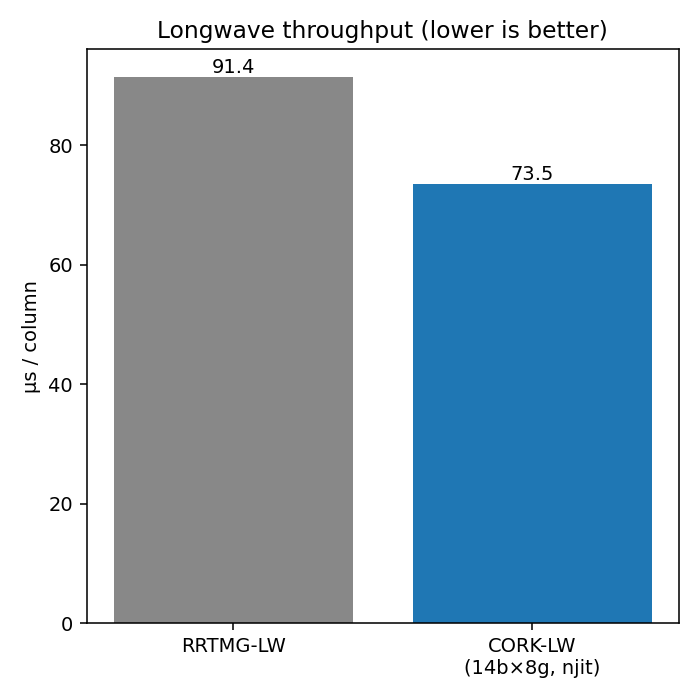
The following figure shows throughput (columns per second) and per-call timing measured with 100 columns × 30 levels in a single process.

Figure 1: Figure A.1 — CORK-LW vs. RRTMG-LW throughput at 100 columns × 30 levels. CORK-LW (14 bands, 8 g-points) achieves 52.9 µs/col against RRTMG-LW’s 63.3 µs/col (0.84× relative wall-clock time — see table below). The profile breakdown shows that the Numba-compiled _ck_tau_additive_co2_kernel dominates the hot path.

Key numbers from that run:

Scheme	ms / call (100 col)	µs / col	vs. RRTMG
RRTMG-LW	6.33 ± 0.02	63.3	1.00×
CORK-LW (14b × 8g)	5.29 ± 0.14	52.9	0.84×

“0.84×” means CORK uses 84% of RRTMG’s wall-clock time — it is faster.

What makes it fast

Numba @njit(parallel=True) with prange

The outermost loop of every hot kernel iterates over columns, which are fully independent. CORK marks those loops with prange and compiles the whole function with @njit(parallel=True). Numba dispatches the column loop to a thread pool (one thread per core) at zero Python overhead.

The optical-depth kernel — the single most expensive function — is _ck_tau_additive_co2_kernel:

import inspect
from climt._components.cork.optics.correlated_k import _ck_tau_additive_co2_kernel
print(inspect.getsource(_ck_tau_additive_co2_kernel))

@njit(parallel=True)
def _ck_tau_additive_co2_kernel(
    k, T_grid, p_grid_log, log_x_grid, log_c_grid,
    Tarr, log_p, log_x, log_c, gas_amounts,
    has_cont, log_cont, co2_logk, tau,
):
    ngas, nband, ngpt = k.shape[0], k.shape[1], k.shape[2]
    nlev = Tarr.shape[0]
    ncol = Tarr.shape[1]
    FLOOR = 1e-40
    for i in prange(ncol):
        for kk in range(nlev):
            iT, fT = _ck_bracket(T_grid, Tarr[kk, i])
            iP, fP = _ck_bracket(p_grid_log, log_p[kk, i])
            iX, fX = _ck_bracket(log_x_grid, log_x[kk, i])
            iC, fC = _ck_bracket(log_c_grid, log_c[kk, i])
            for ib in range(nband):
                if has_cont:
                    lc = _ck_txx_cont(log_cont, ib, iT, fT, iP, fP, iX, fX)
                    cont_val = np.exp(lc)
                else:
                    cont_val = 0.0
                for igp in range(ngpt):
                    acc = 0.0
                    for ig in range(ngas):
                        c0 = _ck_txx7(k, ig, ib, igp, iT, fT, iP, fP, iX, fX, iC)
                        c1 = _ck_txx7(k, ig, ib, igp, iT, fT, iP, fP, iX, fX, iC + 1)
                        if co2_logk:
                            l0 = np.log(c0 if c0 > FLOOR else FLOOR)
                            l1 = np.log(c1 if c1 > FLOOR else FLOOR)
                            kv = np.exp(l0 * (1.0 - fC) + l1 * fC)
                        else:
                            kv = c0 * (1.0 - fC) + c1 * fC
                        acc += kv * gas_amounts[ig, kk, i]
                    if has_cont:
                        acc += cont_val * gas_amounts[0, kk, i]
                    tau[ib, igp, kk, i] = acc

Notice @njit(parallel=True) at the top and for i in prange(ncol) as the outer loop: every column is dispatched to a separate thread.

The same pattern appears in the LW transport kernel:

import inspect
from climt._components.cork.lw.kernels import _lw_transport_kernel
print(inspect.getsource(_lw_transport_kernel))

@njit(parallel=True)
def _lw_transport_kernel(
    tau, planck_source, surface_source, emissivity, weights,
    up_band, down_band, up_broad, down_broad,
    diag_trans, diag_up_gpt, diag_dn_gpt, want_diag, diffusivity_factor,
):
    """Consolidated multi-band, multi-g-point LW transport.

    Loops over columns in parallel; for each (band, g-point) runs the up/down
    diffusivity sweeps and accumulates weighted fluxes into up_band/down_band
    inside the compiled kernel. Accumulation order (g ascending, then b
    ascending for broadband) matches the original python loops bit-for-bit.
    """
    nband, ngpt, nlev, ncol = tau.shape
    for i in prange(ncol):
        for k in range(nlev + 1):
            up_broad[k, i] = 0.0
            down_broad[k, i] = 0.0
        for b in range(nband):
            for k in range(nlev + 1):
                up_band[b, k, i] = 0.0
                down_band[b, k, i] = 0.0
            for g in range(ngpt):
                w = weights[b, g]
                # Upward sweep: surface -> TOA
                up_prev = emissivity[b, i] * surface_source[b, g, i]
                up_band[b, 0, i] += w * up_prev
                if want_diag != 0:
                    diag_up_gpt[b, g, 0, i] = w * up_prev
                for k in range(nlev):
                    trans = np.exp(-diffusivity_factor * tau[b, g, k, i])
                    up_cur = up_prev * trans + planck_source[b, g, k, i] * (1.0 - trans)
                    up_band[b, k + 1, i] += w * up_cur
                    if want_diag != 0:
                        diag_trans[b, g, k, i] = trans
                        diag_up_gpt[b, g, k + 1, i] = w * up_cur
                    up_prev = up_cur
                # Downward sweep: TOA -> surface (dn_prev starts at 0 = TOA BC)
                dn_prev = 0.0
                if want_diag != 0:
                    diag_dn_gpt[b, g, nlev, i] = 0.0
                for k in range(nlev - 1, -1, -1):
                    trans = np.exp(-diffusivity_factor * tau[b, g, k, i])
                    dn_cur = dn_prev * trans + planck_source[b, g, k, i] * (1.0 - trans)
                    down_band[b, k, i] += w * dn_cur
                    if want_diag != 0:
                        diag_dn_gpt[b, g, k, i] = w * dn_cur
                    dn_prev = dn_cur
            for k in range(nlev + 1):
                up_broad[k, i] += up_band[b, k, i]
                down_broad[k, i] += down_band[b, k, i]

Pure-NumPy k-table interpolation; no Python in the hot path

k-table lookup involves a 4-D bilinear interpolation in \((T, p, x_\text{H_2O}, x_\text{CO_2})\) space. The bracket-finding helpers (_ck_bracket) and interpolation helpers (_ck_txx7, _ck_txx_cont) are all @njit-compiled scalar functions. Once Numba has compiled the outer kernel on first call, no Python bytecode executes inside the column/level/band/g-point quadruple loop.

One-time unit conversion in array_call

Reshaping, unit conversion (mole fraction → kg m⁻²), and output unpacking are performed once per component call inside CorkLongwaveRadiation.array_call, before any kernel is invoked. The compiled kernels receive raw NumPy arrays of the correct shape and units and never touch Python objects.

Graceful no-Numba fallback

When Numba is unavailable (e.g. in a Pyodide/WebAssembly context), common.py replaces @njit with a no-op decorator and prange with the built-in range. The scheme still runs correctly in pure Python — just without the multi-threaded speed-up. Interactive notebooks in JupyterLite use this path.

import inspect
from climt._components.cork.common import njit
print(inspect.getsource(njit))

    def njit(*args, **kwargs):
        # No-numba fallback. Support both bare ``@njit`` and parametrized
        # ``@njit(parallel=True, ...)`` usage so the pure-Python path imports.
        if len(args) == 1 and callable(args[0]) and not kwargs:
            return args[0]

        def _decorator(func):
            return func

        return _decorator

Profiling the hot path

The profiler output recorded alongside the benchmark confirms that array_call accounts for essentially the entire call budget, with _correlated_k_optics (k-table lookup) taking the bulk of that:

ncalls  tottime  cumtime  filename:lineno(function)
     1    0.001    0.005   cork/lw/component.py:200(array_call)
     1    0.000    0.002   cork/lw/component.py:415(_correlated_k_optics)
     1    0.000    0.002   cork/optics/correlated_k.py:347(compute_ck_optical_depth)
     1    0.000    0.002   cork/optics/correlated_k.py:447(_compute_ck_optical_depth_additive)
     1    0.000    0.002   cork/optics/correlated_k.py:498(_additive_co2_fast)
     1    0.001    0.001   cork/optics/correlated_k.py:81(_ck_tau_additive_co2_kernel)

The outermost Python frame (array_call) costs 1 ms; the compiled _ck_tau_additive_co2_kernel costs another 1 ms on the reference machine. Everything else is sub-millisecond bookkeeping.

WarningFirst-call JIT latency

Numba compiles each kernel the first time it is called. Expect a 5–30 second pause on the very first CorkLongwaveRadiation.__call__ in a fresh Python process. Subsequent calls are fast. If you are timing CORK in a benchmark, always make a warm-up call before recording.

TipReproduce the benchmark

Run the benchmark script from the repo root (climt environment):

conda run --no-capture-output -n climt python scripts/experiments/bench_cork_vs_rrtmg.py

Pass --save <path>.npz to persist raw timing arrays. This prints the per-call timing and throughput breakdown and saves docs/experiments/2026-06-05-cork-co2-bands/_artifacts/throughput.png.

Heating-rate kernel

The heating-rate calculation uses the same @njit / prange pattern. compute_heating_rate in climt/_components/cork/common.py iterates over columns in parallel:

import inspect
from climt._components.cork.common import compute_heating_rate
print(inspect.getsource(compute_heating_rate))

@njit
def compute_heating_rate(net_flux, p_interface, g, cpd):
    """Compute heating rate (K/s) from net flux divergence.

    Args:
        net_flux: (nlev+1, ncol) upward minus downward flux, W/m^2
        p_interface: (nlev+1, ncol) pressure at interfaces, Pa
        g: gravitational acceleration, m/s^2
        cpd: heat capacity of dry air at constant pressure, J/kg/K

    Returns:
        heating_rate: (nlev, ncol) in K/s
    """
    nlev = net_flux.shape[0] - 1
    ncol = net_flux.shape[1]
    heating_rate = np.zeros((nlev, ncol))
    for i in prange(ncol):
        for k in range(nlev):
            dp = p_interface[k + 1, i] - p_interface[k, i]
            dflux = net_flux[k + 1, i] - net_flux[k, i]
            heating_rate[k, i] = g / cpd * dflux / dp
    return heating_rate

Because heating rates are derived from flux divergence — a simple subtraction per layer — this kernel is negligibly cheap compared with the optical-depth computation.

Further reading

• Pincus et al. (2019) — RRTMGP design paper; discusses the accuracy–efficiency trade-off in production correlated-k codes and the rationale for the g-point ordering used by CORK.
• Lacis and Oinas (1991) — the original correlated-k distribution paper; the mathematical framework CORK implements.
• Lam et al. (2015) — Numba: a JIT compiler for numerical Python. Describes the @njit/prange model used throughout CORK’s hot path.

References

Lacis, A. A., and V. Oinas. 1991. “A Description of the Correlated-k Distribution Method for Modeling Nongray Gaseous Absorption, Thermal Emission, and Multiple Scattering in Vertically Inhomogeneous Atmospheres.” Journal of Geophysical Research 96 (D5): 9027–63. https://doi.org/10.1029/90JD01945.

Lam, Siu Kwan, Antoine Pitrou, and Stanley Seibert. 2015. “Numba: A LLVM-Based Python JIT Compiler.” Proceedings of the Second Workshop on the LLVM Compiler Infrastructure in HPC, LLVM ’15, 1–6. https://doi.org/10.1145/2833157.2833162.

Pincus, R., E. J. Mlawer, and J. S. Delamere. 2019. “Balancing Accuracy, Efficiency, and Flexibility in Radiation Calculations for Dynamical Models.” Journal of Advances in Modeling Earth Systems 11: 3074–89. https://doi.org/10.1029/2019MS001621.