Chapter 2: Line-by-line physics
Every opacity climt uses ultimately traces back to HITRAN: the atlas of spectral lines for each greenhouse gas. A line-by-line (LBL) calculation means evaluating the opacity at enough wavenumbers to resolve every individual line — tens of thousands of points per cm⁻¹, over thousands of cm⁻¹, on a T-p grid. It is expensive.
But you only have to do it once. All of correlated-k is a lossy compression of an LBL calculation.
The Voigt line shape
Each spectral line at rest wavenumber \(\nu_0\) with intensity \(S\) has a profile that is the convolution of two broadening mechanisms:
- Doppler broadening: \(\Delta\nu_D \propto \sqrt{T/M}\) — pure Gaussian, dominant in the upper atmosphere and for light gases.
- Pressure broadening: \(\Delta\nu_L \propto p\) — pure Lorentzian, dominant in the troposphere.
The convolution is the Voigt profile:
\[\phi(\nu) = \frac{y}{\pi}\int_{-\infty}^{\infty} \frac{e^{-t^2}}{y^2 + (x-t)^2}\,dt,\]
with \(x = (\nu-\nu_0)/\Delta\nu_D\), \(y = \Delta\nu_L/\Delta\nu_D\). The absorption cross-section at wavenumber \(\nu\) is the sum over all lines of \(S_i\,\phi_i(\nu)\).
What linepyline does
linepyline (Rodrigo Caballero, GPL-3) wraps a Voigt evaluator around the HITRAN line database. You build an rtm object, ask it for a wavenumber grid, and evaluate the mass absorption coefficient (m²/kg) for a gas at a given (T, p):
import linepyline as lpl

r = lpl.rtm()                                    # HITRAN2024 + MT_CKD by default
nu = r.get_nu_grid(1000.0, 1200.0, 0.01)         # cm⁻¹, 0.01 cm⁻¹ spacing
kappa = r.get_kappa_hitran("H2O", 1000.0, 1200.0, 0.01,
                           p=1.0e5, T=296.0)      # m²/kg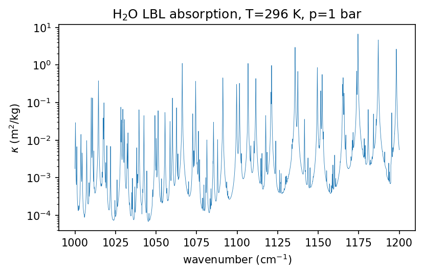
linepyline is an optional dependency. The chapters that use it guard against its absence with a try/except ImportError block. If you see “linepyline not available” in notebook output, install it separately from HITRAN’s line data.
Why not just ship LBL?
A single LBL column from 10 to 30 000 cm⁻¹ at R = 500 000 is ≈ 10⁷ points. Multiply by a T × p grid (14 × 20) and keep one gas in double precision: 22 GB. Three gases: 66 GB. This is why we compress into k-distributions (Chapter 3).
Run examples/k_distribution_demo.ipynb cell by cell. The first half uses linepyline to reproduce Figure 2.1, with a pre-baked fallback array when linepyline is absent.