Chapter 4: Correlated-k
Chapter 3’s k-distribution trick compressed one band at one (T, p). In a real atmosphere opacity depends on (T, p) and gas travels through many layers. If each layer had its own independent k-distribution and the orderings were uncorrelated, we would need to re-integrate the full spectrum at every interface — no cheaper than LBL.
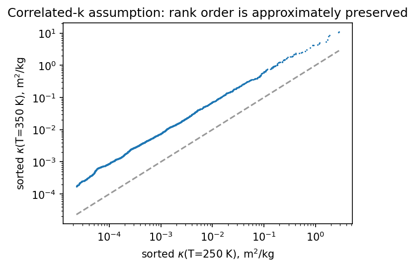
The correlated-k approximation rescues us: for a given g-point, \(k(g)\) varies smoothly with (T, p) but the ranking of opacity values is preserved across layers. The spectral location of the strongest absorber at one level is still the strongest absorber at the next level, just with a different magnitude.
Evidence: how well does ranking hold?
When it holds
- Small-to-moderate temperature variations (~ 100 K): line intensities change smoothly with \(T\) via the Boltzmann factor. ✓
- Pressure variations within a single regime: line widths scale cleanly with \(p\). ✓
- A single well-mixed gas (fixed mixing ratio): the spectral ordering is set by molecular physics alone, independent of (T, p). ✓
When it breaks down
- Very large T ranges spanning new hot-band regimes (e.g., Venus lower troposphere vs. upper atmosphere). Use separate tables per regime.
- Two spectrally independent gases with strongly overlapping line forests — the joint ordering is no longer preserved. Use ESFT overlap instead (Chapter 5).
- Strongly varying mixing ratios (e.g., H₂O in a partly cloudy column). The correlated-k assumption is weakest here; this is one reason RRTMG uses a separate water-vapour continuum fit.
What the approximation gains
With correlated-k, each g-point in each band is an independent quasi-monochromatic problem: the solver sweeps through the column once per (band, g-point) with a single \(k(g)\) value interpolated to local (T, p). No re-ordering needed at runtime.
This is why climt’s tables have layout k(band, gpoint, temperature, pressure): at each (T, p) look-up point the \(k_i(g_i)\) is the same \(g_i\) across the whole column.
Accuracy
Typical broadband flux errors for correlated-k with 8 g-points per band are 1–3 % versus LBL (Lacis and Oinas 1991; Mlawer et al. 1997). The picket-fence tables ship with 2 g-points per band — errors grow to ~5–10 %. That is sufficient for pedagogy and fast prototype runs; earth_high_res with 8 g-points is the recommended production configuration.