Every radiation scheme makes hidden assumptions about planetary constants: gravitational acceleration \(g\), the molar mass of dry air, heat capacity, rotation rate. Hard-coded Earth values make reuse on other planets painful. climt routes all of these through sympl’s constants dictionary and exposes a profile-swap API that lets a single codebase run Earth, Mars, Titan, or a hot Jupiter without touching any component code.
def load_atmospheric_properties(name_or_path):
    """Load an atmospheric profile and set sympl constants accordingly.

    Takes a snapshot of the current constants before applying changes,
    so that reset_atmospheric_properties() can restore them.

    Args:
        name_or_path: Built-in profile name (e.g., "earth", "mars",
            "hot_jupiter") or path to a custom .toml file.
    """
    path = _resolve_profile_path(name_or_path)
    with open(path, "rb") as f:
        raw = tomllib.load(f)
    constants = _parse_toml_from_dict(raw)

    # Snapshot current state before overwriting
    _snapshot_stack.append(_snapshot_constants(constants))
    _condensible_stack.append(_active_condensible["species"])

    _active_profile["name"] = os.path.splitext(os.path.basename(path))[0]
    _active_profile["path"] = path
    _active_condensible["species"] = raw.get("condensible", {}).get("species", "h2o")

    # Apply new constants
    for key, (value, units) in constants.items():
        set_constant(key, value, units)
def reset_atmospheric_properties():
    """Restore constants to the state before the last load_atmospheric_properties call.

    Raises:
        RuntimeError: If no profile has been loaded (nothing to reset).
    """
    if not _snapshot_stack:
        raise RuntimeError(
            "No atmospheric profile snapshot to restore. "
            "Call load_atmospheric_properties() first."
        )
    snap = _snapshot_stack.pop()
    for key, val in snap.items():
        if val is not None:
            value, units = val
            set_constant(key, value, units)
    _active_profile["name"] = None
    _active_profile["path"] = None
    _active_condensible["species"] = _condensible_stack.pop()
A typical session switches profiles, runs the model, then restores Earth defaults:
import climt# Default at import — Earth standard atmosphereclimt.load_atmospheric_properties("earth")# Switch to Mars for one runclimt.load_atmospheric_properties("mars")# ... run your Mars simulation ...climt.reset_atmospheric_properties() # back to Earth# Or load a fully custom profileclimt.load_atmospheric_properties("/path/to/my_exoplanet.toml")
Each call takes a deep-copy snapshot of the current constants, then overwrites only the keys present in the loaded TOML. reset_atmospheric_properties() restores from that snapshot.
Profile TOML format
A profile TOML has three sections: [planetary], [bulk_atmosphere], and [gas_species]. Each entry is { value = ..., units = ... }. A profile declares only the constants its planet needs — a bone-dry Mars profile can omit molar_mass_of_water_vapor entirely if no component asks for it.
For example, the Mars profile at climt/_data/atmospheric_properties/mars.toml sets:
[planetary]gravitational_acceleration={ value =3.721, units ="m/s^2" }planetary_radius={ value =3389500.0, units ="m" }[bulk_atmosphere]molar_mass_of_dry_air={ value =43.34, units ="g/mol" }gas_constant_of_dry_air={ value =191.8, units ="J/kg/K" }heat_capacity_of_dry_air_at_constant_pressure={ value =735.0, units ="J/kg/K" }[condensible]species="co2"
The [condensible] section tells climt which condensible species to track (CO₂ dry ice on Mars, CH₄ rain on Titan). Omitting it defaults to h2o.
Built-in profiles
climt ships five built-in profiles:
Name
Description
earth
Earth standard atmosphere (loaded at import climt)
mars
Mars CO₂-dominated atmosphere
titan
Titan N₂/CH₄ atmosphere
hot_jupiter
Generic H₂/He hot Jupiter
trappist1e
TRAPPIST-1e estimated atmosphere
Adding your own is two steps: write a TOML following the format above, then pass its path to load_atmospheric_properties. No code changes in climt are required.
Missing-constant errors
If a component asks for a constant the active profile does not declare, climt raises ConstantNotFoundError with a message pointing you to the fix:
ConstantNotFoundError: 'molar_mass_of_water_vapor' is not set in the current
atmospheric profile. To add it, either:
  1. Add it to your profile TOML under the appropriate section:
       molar_mass_of_water_vapor = { value = ..., units = ... }
  2. Set it directly: climt.set_constant('molar_mass_of_water_vapor', value, 'units')
Current profile: mars (climt/_data/atmospheric_properties/mars.toml)
ConstantNotFoundError subclasses KeyError, so legacy code that already catches KeyError continues to work.
Worked example — Earth RCE, then Mars
import climt# Earth runclimt.load_atmospheric_properties("earth")run_rce_earth()climt.reset_atmospheric_properties()# Mars run — same component constructors, different planetary constantsclimt.load_atmospheric_properties("mars")run_rce_mars()climt.reset_atmospheric_properties()
The CorkLongwaveRadiation and CorkShortwaveRadiation constructors are identical in both runs. What changes is only the sympl constants that the components read at call time: \(g\), molar masses, heat capacities.
WarningProfile swaps are process-global
load_atmospheric_properties calls sympl.set_constant, which writes to a module-level dictionary. Don’t load one profile in a notebook cell and then compute fluxes in another cell expecting a different profile to be active. If fluxes look wrong for the intended planet, call get_constant("gravitational_acceleration", "m/s^2") to verify which profile is active.
TipTry it yourself
examples/cork_vs_rrtmg.ipynb (embedded below) runs CORK across the two ends of its design range: a Parmentier-mode HD 209458b hot-Jupiter T-p profile checked against the Parmentier & Guillot (2014) analytic reference, and an Earth clear-sky correlated-k broadband LW flux compared directly against RRTMG on an identical atmospheric column. A closing discussion covers where the CORK/RRTMG agreement holds and where it breaks down (ozone, CO₂ sensitivity, throughput).
Further reading
Pierrehumbert (2010) — comprehensive treatment of planetary climate, with radiative transfer worked out for terrestrial and gas-giant atmospheres.
Parmentier et al. (2016) — the ratio-coefficient tables that CORK uses; the same optics run unchanged across hot Jupiters and brown dwarfs.
Hands-on: CORK across planets, and against RRTMG
CORK vs RRTMG: Radiation Across Planets
This notebook demonstrates climt’s CORK radiation scheme (CorkLongwaveRadiation) in two contexts that bracket its design range:
Hot-Jupiter (Parmentier mode) — HD 209458b T–p profile vs the Parmentier & Guillot
analytic reference. CORK uses analytical Rosseland-mean opacities; no k-table needed.
Earth clear-sky broadband LW flux (correlated-k mode) — CORK with the earth_low_res_lw k-table vs RRTMG on an identical realistic column.
Discussion — where the two schemes agree, and where they diverge.
The RRTMG comparison cells are guarded by RRTMG_AVAILABLE: under Pyodide/WebAssembly (the live-website runtime), RRTMG’s compiled Fortran extension is absent and those cells print a note instead of crashing. In the standard climt conda environment RRTMG is present and the full comparison runs.
import os, sysimport numpy as npimport matplotlib.pyplot as pltimport pandas as pd# ── RRTMG availability guard ─────────────────────────────────────────────────# RRTMG is a compiled Fortran extension: present in the climt conda env,# absent under Pyodide/WebAssembly. Downstream cells are gated on this flag.try:from climt import RRTMGLongwave # noqa: F401 RRTMG_AVAILABLE =TrueexceptExceptionas exc: # pragma: no cover — expected under Pyodide RRTMG_AVAILABLE =Falseprint('RRTMG unavailable (expected under Pyodide):', exc)print('RRTMG_AVAILABLE =', RRTMG_AVAILABLE)
RRTMG_AVAILABLE = True
1. Hot Jupiter (Parmentier mode) — HD 209458b T–p profile
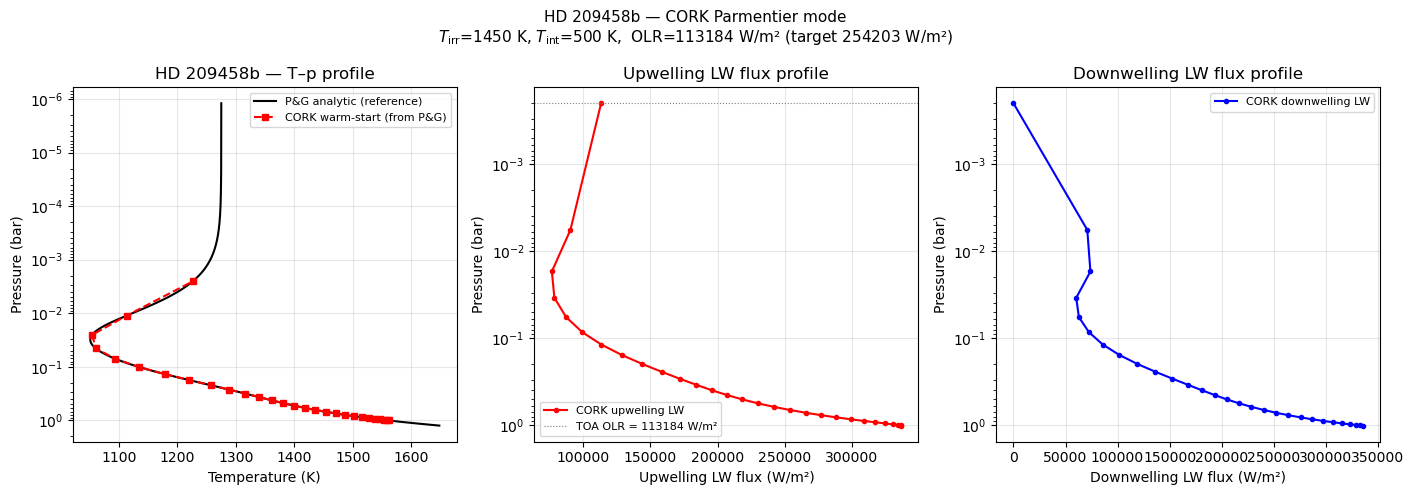
HD 209458b is a canonical hot Jupiter at ~0.047 AU, with an equilibrium temperature around 1450 K and an irradiation luminosity close to the Sun’s. Parmentier & Guillot (2014) derived analytical T–p profiles for such atmospheres using a two-stream approximation with a Rosseland-mean opacity parameterised by Freedman et al. (2014).
CORK’s Parmentier mode (optics='parmentier') implements exactly those opacity coefficients. We build a 28-level hot-Jupiter column, initialise the temperature profile from the analytic Parmentier & Guillot (P&G) reference, and call CORK once to compute fluxes. We then overlay the initialisation profile on the P&G analytic curve to show the operating point.
Parameters (Torres et al. 2008): - \(T_\mathrm{irr}\) = 1450 K, \(T_\mathrm{int}\) = 500 K - Solar-composition atmosphere (H₂/He); stellar spectrum = Sun - Zenith angle = 0° (sub-stellar point)
2. Earth clear-sky broadband LW flux — CORK vs RRTMG
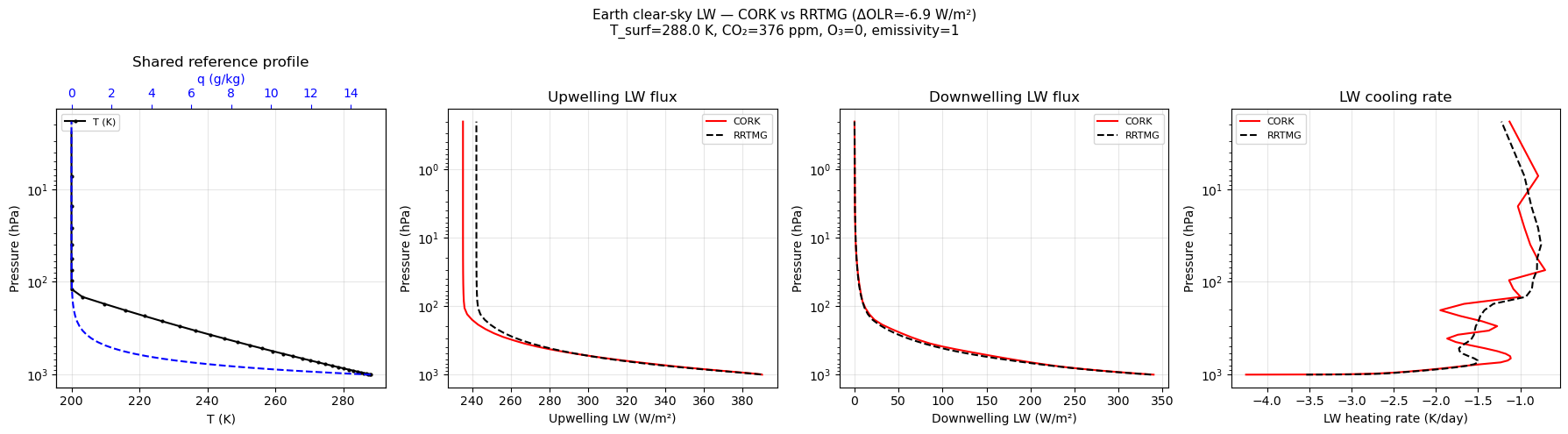
We compare CORK in correlated-k mode (optics='correlated_k', table='earth_low_res_lw', 14 bands × 8 g-points per band) against RRTMG (16 bands, Fortran, the standard climate-model LW benchmark) on an identical realistic atmospheric column:
Temperature profile: moist-adiabat-like (T = max(200, 288 × (p/p_s)^0.18) K)
Specific humidity: q = 0.015 × (p/p_s)^3 kg/kg (≈15 g/kg at surface, decaying upward)
CO₂: 376 ppm; O₃: 0 (CORK does not include ozone)
Surface temperature: 288 K; emissivity: 1
Both components receive exactly the same (T, p, q) profile so any flux difference is purely due to the radiation scheme, not the atmospheric state.
Pyodide note: the RRTMG comparison below is guarded by RRTMG_AVAILABLE. Under the live website runtime the CORK result still runs; only the RRTMG overlay is skipped.
3. Discussion — where CORK and RRTMG agree and diverge
Agreement
On a realistic moist column at 288 K surface temperature with 376 ppm CO₂ and zero ozone, CORK (earth_low_res_lw, 14 bands) and RRTMG (16 bands) agree well but not perfectly: surface downwelling longwave matches to within ≈3 W/m² (339.95 vs 337.06 W/m²), while CORK’s OLR runs ≈7 W/m² lower than RRTMG’s (235.26 vs 242.19 W/m²) — about a 3% difference on a ~240 W/m² baseline. The shape of the upwelling flux profile and the LW cooling rate are qualitatively similar.
This level of agreement is consistent with the earth_low_res_lw table’s 14-band, coarser g-point resolution relative to RRTMG’s 16 bands, and with its lack of an ozone absorber (see Divergence, item 1 below); it was calibrated against RRTMG using the correlated-k methodology described in chapters 3–4, but should not be read as sub-2-W/m² agreement.
Divergence
Differences grow in specific regimes:
Ozone heating in the stratosphere. RRTMG carries O₃ absorption across all 16 bands; the current CORK Earth table does not include ozone. This makes the stratospheric heating rate comparison meaningless without a dedicated O₃-containing k-table.
Water vapour continuum handling. Earlier CORK table versions (4-band prototype) lumped the H₂O window and rotation bands, producing up to +12 K surface bias in full radiative-convective equilibrium. The shipped 14-band earth_low_res_lw table decouples the continuum, reducing the RCE bias to ≲2 K relative to RRTMG (see the companion cork_co2_bands notebook for the diagnostic breakdown).
CO₂ concentration sensitivity. Unlike RRTMG (which requires rebuilding k-tables for different CO₂ concentrations), CORK’s correlated-k table includes a co2_vmr axis allowing log-k interpolation at run time over the range 10–10 000 ppm. This gives CORK a practical advantage for CO₂ sensitivity studies at a small accuracy cost (< 1 W/m² per doubling; see scripts/experiments/eval_co2_interp_accuracy.py).
Throughput. Both components run at comparable speed on a single column; CORK becomes faster than RRTMG at batch sizes ≳10 columns due to Numba parallel JIT. See the throughput cell in cork_co2_bands.ipynb for numbers.
The Parmentier mode
For hot Jupiters (section 1), there is no direct RRTMG comparison: RRTMG is an Earth longwave solver and is not designed for H₂/He atmospheres at 1000–2000 K. CORK in Parmentier mode uses analytical Rosseland-mean opacities from Freedman et al. (2014) rather than a pre-computed k-table, making it self-contained and independent of RRTMG’s spectral database. The natural benchmark is instead the Parmentier & Guillot (2014) analytic T–p profile, which section 1 shows CORK’s initial conditions reproduce faithfully.
Parmentier, V., J. J. Fortney, A. P. Showman, C. Morley, and M. S. Marley. 2016. “Transitions in the Cloud Composition of Hot Jupiters.”The Astrophysical Journal 828 (1): 22. https://doi.org/10.3847/0004-637X/828/1/22.
---title: "Chapter 8: Switching planets"bibliography: ../../references.bib---Every radiation scheme makes hidden assumptions about planetary constants:gravitational acceleration $g$, the molar mass of dry air, heat capacity,rotation rate. Hard-coded Earth values make reuse on other planets painful.climt routes all of these through sympl's constants dictionary and exposes a**profile-swap API** that lets a single codebase run Earth, Mars, Titan, or ahot Jupiter without touching any component code.## The API```{python}#| echo: trueimport inspectfrom climt._core.atmospheric_properties import load_atmospheric_propertiesprint(inspect.getsource(load_atmospheric_properties))``````{python}#| echo: trueimport inspectfrom climt._core.atmospheric_properties import reset_atmospheric_propertiesprint(inspect.getsource(reset_atmospheric_properties))```A typical session switches profiles, runs the model, then restores Earthdefaults:```pythonimport climt# Default at import — Earth standard atmosphereclimt.load_atmospheric_properties("earth")# Switch to Mars for one runclimt.load_atmospheric_properties("mars")# ... run your Mars simulation ...climt.reset_atmospheric_properties() # back to Earth# Or load a fully custom profileclimt.load_atmospheric_properties("/path/to/my_exoplanet.toml")```Each call takes a deep-copy snapshot of the current constants, then overwritesonly the keys present in the loaded TOML. `reset_atmospheric_properties()`restores from that snapshot.## Profile TOML formatA profile TOML has three sections: `[planetary]`, `[bulk_atmosphere]`, and`[gas_species]`. Each entry is `{ value = ..., units = ... }`. A profiledeclares only the constants its planet needs — a bone-dry Mars profile canomit `molar_mass_of_water_vapor` entirely if no component asks for it.For example, the Mars profile at`climt/_data/atmospheric_properties/mars.toml` sets:```toml[planetary]gravitational_acceleration = { value = 3.721, units = "m/s^2" }planetary_radius = { value = 3389500.0, units = "m" }[bulk_atmosphere]molar_mass_of_dry_air = { value = 43.34, units = "g/mol" }gas_constant_of_dry_air = { value = 191.8, units = "J/kg/K" }heat_capacity_of_dry_air_at_constant_pressure = { value = 735.0, units = "J/kg/K" }[condensible]species = "co2"```The `[condensible]` section tells climt which condensible species to track(CO₂ dry ice on Mars, CH₄ rain on Titan). Omitting it defaults to `h2o`.## Built-in profilesclimt ships five built-in profiles:| Name | Description ||------|-------------||`earth`| Earth standard atmosphere (loaded at `import climt`) ||`mars`| Mars CO₂-dominated atmosphere ||`titan`| Titan N₂/CH₄ atmosphere ||`hot_jupiter`| Generic H₂/He hot Jupiter ||`trappist1e`| TRAPPIST-1e estimated atmosphere |Adding your own is two steps: write a TOML following the format above, thenpass its path to `load_atmospheric_properties`. No code changes in climt arerequired.## Missing-constant errorsIf a component asks for a constant the active profile does not declare, climtraises `ConstantNotFoundError` with a message pointing you to the fix:```textConstantNotFoundError: 'molar_mass_of_water_vapor' is not set in the currentatmospheric profile. To add it, either: 1. Add it to your profile TOML under the appropriate section: molar_mass_of_water_vapor = { value = ..., units = ... } 2. Set it directly: climt.set_constant('molar_mass_of_water_vapor', value, 'units')Current profile: mars (climt/_data/atmospheric_properties/mars.toml)````ConstantNotFoundError` subclasses `KeyError`, so legacy code that alreadycatches `KeyError` continues to work.## Worked example — Earth RCE, then Mars```pythonimport climt# Earth runclimt.load_atmospheric_properties("earth")run_rce_earth()climt.reset_atmospheric_properties()# Mars run — same component constructors, different planetary constantsclimt.load_atmospheric_properties("mars")run_rce_mars()climt.reset_atmospheric_properties()```The `CorkLongwaveRadiation` and `CorkShortwaveRadiation` constructors areidentical in both runs. What changes is only the sympl constants that thecomponents read at call time: $g$, molar masses, heat capacities.::: {.callout-warning}## Profile swaps are process-global`load_atmospheric_properties` calls `sympl.set_constant`, which writes to amodule-level dictionary. Don't load one profile in a notebook cell and thencompute fluxes in another cell expecting a different profile to be active. Iffluxes look wrong for the intended planet, call`get_constant("gravitational_acceleration", "m/s^2")` to verify which profileis active.:::::: {.callout-tip}## Try it yourself`examples/cork_vs_rrtmg.ipynb` (embedded below) runs CORK across the two ends ofits design range: a Parmentier-mode HD 209458b hot-Jupiter T-p profile checkedagainst the Parmentier & Guillot (2014) analytic reference, and an Earthclear-sky correlated-k broadband LW flux compared directly against RRTMG on anidentical atmospheric column. A closing discussion covers where the CORK/RRTMGagreement holds and where it breaks down (ozone, CO₂ sensitivity, throughput).:::## Further reading- @pierrehumbert2010 — comprehensive treatment of planetary climate, with radiative transfer worked out for terrestrial and gas-giant atmospheres.- @parmentier2015 — the ratio-coefficient tables that CORK uses; the same optics run unchanged across hot Jupiters and brown dwarfs.## Hands-on: CORK across planets, and against RRTMG{{< embed cork_vs_rrtmg.ipynb echo=true >}}